Pandas - practical example: portfolio activity
Elements of Pandas explained in the article:
- DataFrame - The most important object in the pandas library.
- Common DataFrame functions: head(), info(), read_csv(), copy(), to_date(), astype(), index(), to_datetime(), dt.normalize(), insert(), pop(), to_numeric(), unique(), sum(), drop(), rename(), round()
- Boolean Masking: A filtering technique for selecting specific data.
- Column Calculations: Performing operations on DataFrame columns.
- Merging Tables: Combining data from multiple DataFrames.
- Date Manipulation: Working with and modifying date values.

The files used in this example, along with the Jupyter Notebook project file containing the full explanation and code, can be found at the following link in my GitHub repository: https://github.com/analysislessons/Article_PandasPortfolioActivity
We are investigating the profits of a beginner investor on U.S. stock exchanges and have reached a surprising conclusion.
First, we need to import the pandas library into our project. This can be done with a single line of code, as shown below. However, before importing, it’s necessary to install the library.
Secondly, we need to upload the data into our project. Our dataset is stored in a spreadsheet named TRANSACTIONS.xlsx, in a sheet called data. The data is structured as a table and is loaded into a DataFrame using pandas.
**In pandas, there are two main data structures:
Series – used for handling one-dimensional data (a single row or column)
DataFrame – used for working with tabular data (tables with rows and columns)**
We named the structure df_transactions, where the prefix 'df' stands for 'DataFrame', indicating the type of the structure. Now, using the head() function, we can view the column headers and the first five rows of our data. You can also display any number of rows by passing a specific number to the head() function—for example, head(10) will show the first 10 rows.
| Quantity | Symbol | Exchange Code | Open Time | Close Time | Open Price | Close Price | Currency | Cash Operation | |
|---|---|---|---|---|---|---|---|---|---|
| 0 | 10.0000 | NVDA.US | XNAS | 2024-10-15 16:58:37.174 | 2024-10-15 17:14:08.928 | 131.89 | 132.11 | USD | Close Trade |
| 1 | 0.2107 | SMCI.US | XNAS | 2024-10-30 16:21:39.160 | 2024-10-30 20:24:19.077 | 34.15 | 33.90 | USD | Close Trade |
| 2 | 39.7893 | SMCI.US | XNAS | 2024-10-30 16:21:39.591 | 2024-10-30 20:24:19.077 | 34.13 | 33.90 | USD | Close Trade |
| 3 | 11.0000 | MS.US | XNYS | 2024-10-16 15:34:04.240 | 2024-10-16 16:05:44.713 | 118.36 | 120.72 | USD | Close Trade |
| 4 | 0.0860 | TSLA.US | XNAS | 2024-09-20 19:31:15.726 | 2024-09-23 15:30:03.684 | 238.46 | 242.63 | USD | Close Trade |
Now we can review all the column headers and their contents:
- Quantity – The number of stocks involved in the transaction.
- Symbol – The ticker symbol of the company whose stocks were bought or sold.
- Exchange Code – The stock exchange code (e.g., NASDAQ or New York Stock Exchange).
- Open Time – The exact timestamp when the stocks were bought. In our later analysis, we’ll use only the date portion.
- Close Time – The exact timestamp when the stocks were sold.
- Open Price – The price per stock at the time of purchase.
- Close Price – The price per stock at the time of sale.
- Currency – The currency used in the transaction. In our case, all transactions are in USD.
- Cash Operation – The type of operation. In this dataset, there are two types: 'Close Trade' and 'Sec Fee'.
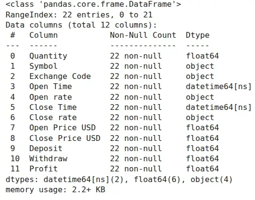
By using the info() function from above, we can obtain information about the number of rows in each column and the data types of the columns.
To clean the dataset, we will first remove the rows labeled 'Sec Fee' and then drop the entire 'Cash Operation' column.
SEC Fee – The Securities and Exchange Commission (SEC) fee is a regulatory charge applied to stock sales (but not buys), paid to the U.S. government. As of 2024, the fee is 8.00 USD per 1,000,000 USD of sale proceeds, which equates to 0.0008%.
The above instruction removed all rows from the dataset where the 'Cash Operation' column was labeled 'Sec Fee'.
The expression df_transactions['Cash Operation'] != 'Sec Fee' is a boolean mask that evaluates to True for rows where the 'Cash Operation' is not equal to 'Sec Fee'. This boolean mask is then placed inside df_transactions[], effectively removing all rows where the mask evaluates to False.
The final step to save the result was to reassign it to df_transactions. This is because df_transactions[...] returns the filtered rows but doesn't modify the original df_transactions object. Without reassigning, df_transactions would remain unchanged.
The following line ensures that all rows labeled 'Sec Fee' were removed, as the unique() function returns all unique values from the 'Cash Operation' column. As a result, we can see that only 'Close Trade' remains.
Now, we can drop the entire 'Cash Operation' column
We will also add 'USD' to the column headers of Open Price and Close Price to avoid future confusion.
| Quantity | Symbol | Exchange Code | Open Time | Close Time | Open Price USD | Close Price USD | Currency | |
|---|---|---|---|---|---|---|---|---|
| 0 | 10.0000 | NVDA.US | XNAS | 2024-10-15 16:58:37.174 | 2024-10-15 17:14:08.928 | 131.89 | 132.11 | USD |
| 1 | 0.2107 | SMCI.US | XNAS | 2024-10-30 16:21:39.160 | 2024-10-30 20:24:19.077 | 34.15 | 33.90 | USD |
Next, we will calculate the total result for the investor in 2024.
First, we’ll add two columns:
- 'Deposit' – the value of the invested capital when the stocks were bought: Quantity × Open Price.
- 'Withdraw' – the value of the stocks when the position was closed: Quantity × Close Price.
| Quantity | Symbol | Exchange Code | Open Time | Close Time | Open Price USD | Close Price USD | Currency | Deposit | Withdraw | |
|---|---|---|---|---|---|---|---|---|---|---|
| 0 | 10.0000 | NVDA.US | XNAS | 2024-10-15 16:58:37.174 | 2024-10-15 17:14:08.928 | 131.89 | 132.11 | USD | 1318.900000 | 1321.10000 |
| 1 | 0.2107 | SMCI.US | XNAS | 2024-10-30 16:21:39.160 | 2024-10-30 20:24:19.077 | 34.15 | 33.90 | USD | 7.195405 | 7.14273 |
As you can see, the Deposit and Withdraw columns have many decimal places. We can easily round them to two decimal places using the round() function:
| Quantity | Symbol | Exchange Code | Open Time | Close Time | Open Price USD | Close Price USD | Currency | Deposit | Withdraw | |
|---|---|---|---|---|---|---|---|---|---|---|
| 0 | 10.0000 | NVDA.US | XNAS | 2024-10-15 16:58:37.174 | 2024-10-15 17:14:08.928 | 131.89 | 132.11 | USD | 1318.9 | 1321.10 |
| 1 | 0.2107 | SMCI.US | XNAS | 2024-10-30 16:21:39.160 | 2024-10-30 20:24:19.077 | 34.15 | 33.90 | USD | 7.2 | 7.14 |
Next, we’ll add one more column, 'Profit', which is the difference between the invested deposit and the withdraw for each transaction. This column will be used to calculate the total result.
We can see that the investor lost 43.75 USD on his investments.
In terms of taxation, due to the negative result, the investor wouldn't need to pay taxes. However, if we assume the investor is based in another country, the situation might be different, since exchange rates fluctuate over time, which could lead to discrepancies. Let's examine this.
Assume the investor pays taxes in Poland. In this case, each transaction will need to be converted from USD to PLN. To do this, we need to upload another table that includes the currency exchange rates.
We upload the table from the file PLN_exchange_rates_2024.csv into a DataFrame, which we call 'rates'. This file contains official currency exchange rates and is in CSV format, which requires us to use the read_csv() function. We must specify the separator used in the file, which is a semicolon (;), so we provide the second argument as sep=';'. Additionally, different countries may use different number formats, so we explicitly define the correct decimal separator for this file, which is a comma (,) by setting decimal=','. If the file uses a different encoding than the default (e.g., UTF-8), we need to specify it explicitly, which in this case is encoding='latin1'.
| data | 1THB | 1USD | 1AUD | 1HKD | 1CAD | 1NZD | 1SGD | 1EUR | 100HUF | 1CHF | 1GBP | 1UAH | 100JPY | 1CZK | 1DKK | 100ISK | 1NOK | 1SEK | 1RON | 1BGN | 1TRY | 1ILS | 100CLP | 1PHP | 1MXN | 1ZAR | 1BRL | 1MYR | 10000IDR | 100INR | 100KRW | 1CNY | 1XDR | nr tabeli | pe³ny numer tabeli | Unnamed: 36 | |
|---|---|---|---|---|---|---|---|---|---|---|---|---|---|---|---|---|---|---|---|---|---|---|---|---|---|---|---|---|---|---|---|---|---|---|---|---|---|
| 0 | NaN | bat (Tajlandia) | dolar amerykañski | dolar australijski | dolar Hongkongu | dolar kanadyjski | dolar nowozelandzki | dolar singapurski | euro | forint (Wêgry) | frank szwajcarski | funt szterling | hrywna (Ukraina) | jen (Japonia) | korona czeska | korona duñska | korona islandzka | korona norweska | korona szwedzka | lej rumuñski | lew (Bu³garia) | lira turecka | nowy izraelski szekel | peso chilijskie | peso filipiñskie | peso meksykañskie | rand (Republika Po³udniowej Afryki) | real (Brazylia) | ringgit (Malezja) | rupia indonezyjska | rupia indyjska | won po³udniowokoreañski | yuan renminbi (Chiny) | SDR (MFW) | NaN | NaN | NaN |
| 1 | 20240102 | 0,1155 | 3,9432 | 2,6897 | 0,5046 | 2,9752 | 2,4884 | 2,9809 | 4,3434 | 1,1365 | 4,6596 | 5,0152 | 0,1035 | 2,7855 | 0,1760 | 0,5826 | 2,8898 | 0,3873 | 0,3911 | 0,8737 | 2,2207 | 0,1329 | 1,0919 | 0,4486 | 0,0708 | 0,2330 | 0,2153 | 0,8125 | 0,8567 | 2,5489 | 4,7327 | 0,3032 | 0,5525 | 5,2882 | 1.0 | 001/A/NBP/2024 | NaN |
| 2 | 20240103 | 0,1162 | 3,9909 | 2,6932 | 0,5112 | 2,9947 | 2,4961 | 3,0074 | 4,3646 | 1,1462 | 4,6873 | 5,0397 | 0,1047 | 2,7977 | 0,1770 | 0,5852 | 2,8962 | 0,3844 | 0,3899 | 0,8776 | 2,2316 | 0,1342 | 1,0974 | 0,4510 | 0,0718 | 0,2341 | 0,2132 | 0,8105 | 0,8618 | 2,5781 | 4,7914 | 0,3050 | 0,5585 | 5,3351 | 2.0 | 002/A/NBP/2024 | NaN |
| 3 | 20240104 | 0,1152 | 3,9684 | 2,6760 | 0,5083 | 2,9785 | 2,4849 | 2,9900 | 4,3525 | 1,1468 | 4,6718 | 5,0481 | 0,1044 | 2,7583 | 0,1766 | 0,5835 | 2,8920 | 0,3858 | 0,3885 | 0,8752 | 2,2254 | 0,1329 | 1,0869 | 0,4505 | 0,0715 | 0,2336 | 0,2130 | 0,8065 | 0,8563 | 2,5619 | 4,7676 | 0,3036 | 0,5552 | 5,3260 | 3.0 | 003/A/NBP/2024 | NaN |
| 4 | 20240105 | 0,1148 | 3,9850 | 2,6627 | 0,5101 | 2,9797 | 2,4778 | 2,9925 | 4,3484 | 1,1498 | 4,6714 | 5,0440 | 0,1047 | 2,7443 | 0,1764 | 0,5830 | 2,8893 | 0,3859 | 0,3880 | 0,8742 | 2,2233 | 0,1335 | 1,0824 | 0,4483 | 0,0717 | 0,2340 | 0,2122 | 0,8136 | 0,8562 | 2,5682 | 4,7907 | 0,3023 | 0,5569 | 5,3070 | 4.0 | 004/A/NBP/2024 | NaN |
Take a look at this file: it contains information about 36 different currency exchange rates, but we only need two columns: data and 1USD. Using the instruction below, we’ll remove the other columns.
| data | 1USD | |
|---|---|---|
| 0 | NaN | dolar amerykañski |
| 1 | 20240102 | 3,9432 |
| 2 | 20240103 | 3,9909 |
| 3 | 20240104 | 3,9684 |
| 4 | 20240105 | 3,9850 |
| data | 1USD | |
|---|---|---|
| 251 | 20241230 | 4,0960 |
| 252 | 20241231 | 4,1012 |
| 253 | kod ISO | USD |
| 254 | nazwa waluty | dolar amerykañski |
| 255 | liczba jednostek | 1 |
Now, we have only the necessary columns in the rates data frame, which we'll use. In the main data frame containing all transactions, we retain two columns: 'Deposit' and 'Withdraw', based on which we calculated the total profit in USD. Our goal now is to recalculate these columns in PLN instead of USD, as this method is required for tax calculation purposes.
For each investment transaction, we need two currency exchange rates: one for the 'Open date' and another for the 'Close date'. To successfully add the currency exchange rates from the rates data frame to the main data frame, we need to modify the rates data frame by making two adjustments:
1. Remove rows 0, 253, 254, and 255, as they are inconsistent with the other rows.
2. Convert the date format in the 'data' column. Currently, the column is of object data type, which means it’s not recognized as a date but rather as text. We need to convert it to a proper date format to match the dates in the main data frame.
The to_datetime() function from above converts the string data type to the datetime64 data type, which is the date format used in the main data frame. The format '%Y%m%d' tells the to_datetime() function how to properly interpret the string:
- %Y: 4-digit year (e.g., 2025)
- %m: 2-digit month (e.g., 05)
- %d: 2-digit day (e.g., 01)
Now, all the columns with dates are in the same data type: datetime64. However, the time differs, which makes merging impossible. Since, for currency conversion purposes in tax calculations, only the date (not the time) is important, we will normalize all the dates using the dt.normalize() function. This will set the time for all dates to 00:00:00, while preserving the datetime64 data type.
The following instruction assigns the result of merging df_transactions with df_rates to df_transactions.
As you can see, the merge() function was used on df_transactions, where we joined df_rates.
df_transactions is considered the left table, while df_rates is the right table.
When merging, we must specify two things:
1. Which columns from the left and right tables we will use to pair rows: left_on='Open Time' means that we are using the 'Open Time' column from the df_transactions table, while right_on='data' means we are using the 'data' column from the df_rates table.
2. We need to specify the type of join. In this case, how='left' means we've chosen a left join — for each row in the left table, we try to find a matching row in the right table. As a result of this join type, all rows from the left table will be present after merging, but only those from the right table that could be paired with rows from the left table will be included.
| Quantity | Symbol | Exchange Code | Open Time | Close Time | Open Price USD | Close Price USD | Currency | Deposit | Withdraw | Profit | data | 1USD | |
|---|---|---|---|---|---|---|---|---|---|---|---|---|---|
| 0 | 10.0000 | NVDA.US | XNAS | 2024-10-15 | 2024-10-15 | 131.89 | 132.11 | USD | 1318.90 | 1321.10 | 2.20 | 2024-10-15 | 3,9332 |
| 1 | 0.2107 | SMCI.US | XNAS | 2024-10-30 | 2024-10-30 | 34.15 | 33.90 | USD | 7.20 | 7.14 | -0.06 | 2024-10-30 | 3,9989 |
| 2 | 39.7893 | SMCI.US | XNAS | 2024-10-30 | 2024-10-30 | 34.13 | 33.90 | USD | 1358.01 | 1348.86 | -9.15 | 2024-10-30 | 3,9989 |
| 3 | 11.0000 | MS.US | XNYS | 2024-10-16 | 2024-10-16 | 118.36 | 120.72 | USD | 1301.96 | 1327.92 | 25.96 | 2024-10-16 | 3,9468 |
| 4 | 0.0860 | TSLA.US | XNAS | 2024-09-20 | 2024-09-23 | 238.46 | 242.63 | USD | 20.51 | 20.87 | 0.36 | 2024-09-20 | 3,8317 |
As you can see above, two columns from df_rates were added. You can also observe that the dates for each row were properly paired: the date in the Open Time column matches the date in the data column for each row. For instance, in the row with index 0, both columns show the date '2024-10-15'.
To keep df_transactions as readable as possible, we’ll reorder the columns to place the Open rate column next to the Open Time column. Then, we’ll remove the data column using the pop() function.
| Quantity | Symbol | Exchange Code | Open Time | Open rate | Close Time | Open Price USD | Close Price USD | Currency | Deposit | Withdraw | Profit | data | |
|---|---|---|---|---|---|---|---|---|---|---|---|---|---|
| 0 | 10.0000 | NVDA.US | XNAS | 2024-10-15 | 3,9332 | 2024-10-15 | 131.89 | 132.11 | USD | 1318.90 | 1321.10 | 2.20 | 2024-10-15 |
| 1 | 0.2107 | SMCI.US | XNAS | 2024-10-30 | 3,9989 | 2024-10-30 | 34.15 | 33.90 | USD | 7.20 | 7.14 | -0.06 | 2024-10-30 |
| 2 | 39.7893 | SMCI.US | XNAS | 2024-10-30 | 3,9989 | 2024-10-30 | 34.13 | 33.90 | USD | 1358.01 | 1348.86 | -9.15 | 2024-10-30 |
| 3 | 11.0000 | MS.US | XNYS | 2024-10-16 | 3,9468 | 2024-10-16 | 118.36 | 120.72 | USD | 1301.96 | 1327.92 | 25.96 | 2024-10-16 |
| 4 | 0.0860 | TSLA.US | XNAS | 2024-09-20 | 3,8317 | 2024-09-23 | 238.46 | 242.63 | USD | 20.51 | 20.87 | 0.36 | 2024-09-20 |
In exactly the same way, we'll merge the currency exchange rates from the df_rates table using the dates from the Close Time column. Then, we’ll reorder the columns accordingly.
As you can see above, the newly added columns Open rate and Close rate have an object data type. This suggests that pandas doesn't recognize them as numeric values. The reason for this is that a comma was used as the decimal separator in the table with exchange rates, instead of a dot.
We must fix this issue before using these columns in further calculations. First, the replace() function will replace commas with dots in each column. However, this alone won't be enough to change the data type. After replacing the commas, we'll use the to_numeric() function, which will convert the object data type to float64.
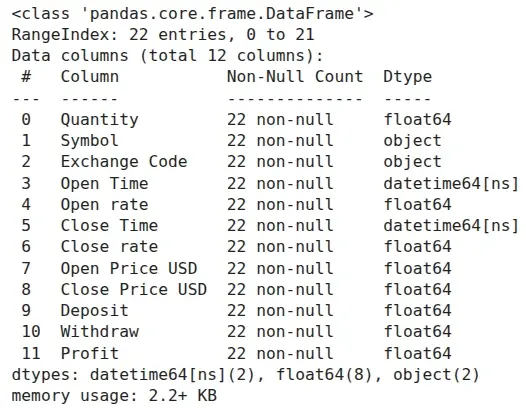
As you can see above, after our modifications, the data type for each exchange rate column is now float64.
Now, we can calculate the values in PLN for each transaction's starting deposit and final withdrawal. We simply multiply the exchange rate by the number of stocks and the stock prices, adding two new columns: Deposit PLN and Withdraw PLN
| Quantity | Symbol | Exchange Code | Open Time | Open rate | Close Time | Close rate | Open Price USD | Close Price USD | Currency | Deposit | Withdraw | Profit | Deposit PLN | Withdraw PLN | |
|---|---|---|---|---|---|---|---|---|---|---|---|---|---|---|---|
| 0 | 10.0000 | NVDA.US | XNAS | 2024-10-15 | 3.9332 | 2024-10-15 | 3.9332 | 131.89 | 132.11 | USD | 1318.90 | 1321.10 | 2.20 | 5187.497480 | 5196.150520 |
| 1 | 0.2107 | SMCI.US | XNAS | 2024-10-30 | 3.9989 | 2024-10-30 | 3.9989 | 34.15 | 33.90 | USD | 7.20 | 7.14 | -0.06 | 28.773705 | 28.563063 |
| 2 | 39.7893 | SMCI.US | XNAS | 2024-10-30 | 3.9989 | 2024-10-30 | 3.9989 | 34.13 | 33.90 | USD | 1358.01 | 1348.86 | -9.15 | 5430.541426 | 5393.945337 |
| 3 | 11.0000 | MS.US | XNYS | 2024-10-16 | 3.9468 | 2024-10-16 | 3.9468 | 118.36 | 120.72 | USD | 1301.96 | 1327.92 | 25.96 | 5138.575728 | 5241.034656 |
| 4 | 0.0860 | TSLA.US | XNAS | 2024-09-20 | 3.8317 | 2024-09-23 | 3.8571 | 238.46 | 242.63 | USD | 20.51 | 20.87 | 0.36 | 78.578818 | 80.482943 |
The instruction above added a new column, Profit PLN, which shows the profits in PLN for each transaction. Now, we can calculate the total profit for the entire year of 2024 for this investor in PLN. To do this, we use the sum() function on the Profit PLN column and round the result to two decimal places:
As you can see total profit in PLN is positive: 93.85 PLN
The investor must pay tax on a profit of 93.85 PLN, which is calculated in accordance with tax regulations. The conclusion is that when making investments, you must consider currency exchange risk, along with other factors.